PyMOL is a great tool for visualising 3D structures of molecules and proteins. It is open-source and can be easily extended using Python code. And as it is open-source you can base your code on existing functionality. This small tutorial will extend the existing half-sphere exposure (HSE) algorithm from a simple discrete count base to a continuous measurement.
The HSE measure
The HSE measure is an indicator for how buried an amino acid residue is within the protein. It simply counts the amino acid neighbours within a half sphere of a given radius. The sphere is divided vertically to the amino acid residue, the $C\alpha$-$C\beta$ vector.
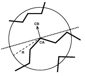
The HSE measure is a very simple discrete measure and will be the subject of our small plugin. We will extend the code to a continuous HSExposure measure which takes distance effects and the search radius into account.
HSExposure in continuous space
Counting neighbours within a half-sphere is a highly simplified approach and there are features of interest which are not taken into account e.g. the sphere radius or the distance of the neighbour residue. There are also disadvantages which come with the discrete space of a simple count algorithm because a continuous variable is much easier translatable into a probabilistic model. The original HSE code already does most of the work and we will simply extend it for our own needs. This is clearly an advantage of open-source.
The scoring function we will use is defined as follows: \[ s(\text{neighbour}) = \frac{1}{\text{radius}} * w(\text{dist}) \] with the following weights \[ w(\text{dist}) = \frac{4}{1+\exp{\sqrt{10d}-6}} \] This weight function describes a sigmoid function with a flatter gradient for higher values due to the non-linear root. This function was simply chosen because it seemed to perform well for a search radius of 12A.
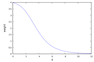
The result of the weight-function are high values for very close residues and low values for distant residues which means that an amino-acid is more buried by close residues than by distant ones. On the other hand, a residue in a very big sphere counts less than in a smaller sphere by dividing the weight by the sphere radius. This can be interpreted as a residue per volume approach because the radius is the only independent variable of the sphere volume. It also scales the sum of all weights within the sphere so that the algorithm performs well in a high range of different sphere radii.
The Python code
The main code of the extension is based on the Bio.PDB.HSExposure module. To reuse the classes in the Bio.PDB module small changes are necessary to make the original code more object orientated by defining a additional function called _add_neighbor() and making the AbstractHSExposure class globally available. The final hse_extended class does the continuous space calculation by inheriting from the imported HSExposure.py.
class hse_extended(AbstractHSExposure,HSExposureCA,HSExposureCB):
    """ this class extends the Bio.PDB.HSExposure.HSExposure class """

    def __init__(self, model, radius, offset):
        """ the hse_extended class is based on HSExposure """
        AbstractHSExposure.__init__(self,model,radius,offset,'EXP_HSE_B_U','EXP_HSE_B_D')

    def _add_neighbor(self,count,d):
        """
        measures the residue per radius instead of a integer quantity of neighbors
        """
        from math import exp
        return count + ((1.0/radius) * (4.0/(1.0+exp(sqrt(10*d.norm())-6))))

    def _get_cb(self, r1, r2, r3):
        if vector_method == 'CA' :
            return HSExposureCA._get_cb(self,r1,r2,r3)
        elif vector_method == 'CB' :
            return HSExposureCB._get_cb(self,r1,r2,r3)
The hse-extended class performing the HSE calculation in continuous space.
Normalisation
There is a typical problem with the two half-spheres approach: The upper sphere requires a normalisation because the side chain spans into the upper half-sphere. Hence, the upper sphere usually has less neighbour residues which are in general also more distant than neighbour residues in the lower sphere. But when we think of the residues per volume approach the accessible volume of the upper sphere is smaller which means that the amino acid is also with less and more distant neighbour residues quite buried.</p>
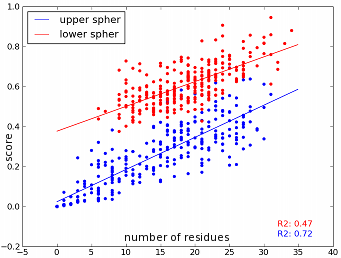
before normalisation
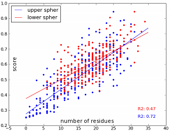
after normalisation
The method shows a overall linear correlation between the number of residues and the continuous score but it also shows that there are great variations within a group of the same amount of neighbour residues.
Modifying the PDB files
The later visualisation in Pymol makes is necessary to renumber the residues in the PDB file because the CA vector method is not applyable to the first and the last residue. Thus, the PDB files are pre-processed in which residues are renumbered and heteroatoms are detached.
Known problems
- The visualisation script works only if there are scores for all residues. This is not the case for smaller radii as no score is calculated if no neighbour residue is present within the sphere.
- The scoring function performs best at 12A. The performance for other radii can be increased with scoring functions which produce a more linear correlation between residue number and residue score e.g. \[ s = \frac{1}{\text{radius}} * 0.8\exp{(-0.1\,d)} \]
Results
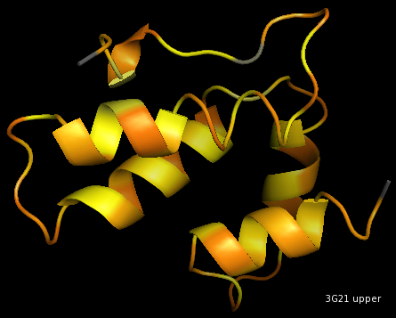
upper sphere
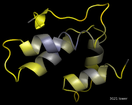
lower sphere
Visualisation of 3G21, 12A, CA-method.
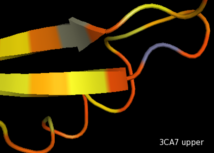
upper sphere
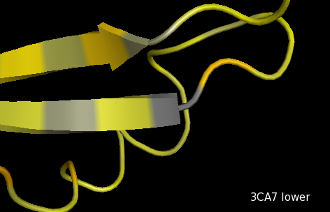
lower sphere
Visualisation of 3CA7, 12A, CA-method
CODE
#!/usr/bin/python
# -*- coding: utf-8 -*-

# hse.py by Jan Teichmann
# date: 15/01/2010

"""
	Calculates the half-spher exposure in Continuous space based
        on a radius weighted distance weight.

        Command Line Arguments: 1)PDB-ID 2)radius 3)CA-CB-vector method
        Example: python hse.py 2PTC 12 CA

        @PDB-ID: 4 letter PDB-database ID
        @radius: float
        @CA-CB-vector method: either CA or CB
"""

from Bio.PDB import PDBList, PDBParser, PDBIO
import sys
from HSExposure import *
from pylab import *


class protein(PDBList,PDBParser):
    """
    creats a new protein-structure object
    """
    def __init__(self,ID):
        """
        initializes the protein class by fetching the pdb file and parsing the structure
        """
        self.pdb = PDBList().retrieve_pdb_file(ID)
        self.structure = PDBParser().get_structure(ID, self.pdb)

class hse_extended(AbstractHSExposure,HSExposureCA,HSExposureCB):
    """ this class extends the Bio.PDB.HSExposure.HSExposureCB class """

    def __init__(self, model, radius, offset):
        """ the hse_extended class is based on HSExposureCB """
        AbstractHSExposure.__init__(self, model, radius, offset, 'EXP_HSE_B_U', 'EXP_HSE_B_D')

    def _add_neighbor(self,count,d):
        """
        measures the residue per radius instead of a integer quantity of neighbors
        """
        from math import exp
        return count + ( ( 1.0 / radius ) * ( 4.0/(1.0 + exp( sqrt(10*d.norm() ) - 6)) ))

    def _get_cb(self, r1, r2, r3):
        if vector_method == 'CA' :
            return HSExposureCA._get_cb(self,r1,r2,r3)
        elif vector_method == 'CB' :
            return HSExposureCB._get_cb(self,r1,r2,r3)

def evaluation(hse, hse_2):
    """
    performs a normalization of the upper spher values and writes the
    results into a text-file which is read by the Pymol visualization script.
    """
    from scipy import stats

    result_u = []
    result_d = []
    result_u_2 = []
    result_d_2 = []
    count = 0

    # read the HSExposure values and rearrange them to a list
    for i in hse:
        count += 1
        result_u.append(  i[1][0] )
        result_d.append(  i[1][1] )

    for ii in hse_2:
        result_u_2.append( ii[1][0] )
        result_d_2.append( ii[1][1] )

    # linear regression
    gradient_u, intercept_u, r_value_u, p_value_u, std_err_u =  \
                stats.linregress(result_u_2, result_u)
    gradient_d, intercept_d, r_value_d, p_value_d, std_err_d =  \
                stats.linregress(result_d_2, result_d)

    #normalization
    corr = 0
    corr = (intercept_d -intercept_u ) - 0.8*max(result_d_2)*abs(gradient_u - gradient_d)
    result_u = result_u + corr

    f1 = open('upper.txt', 'w')
    f2 = open('lower.txt', 'w')

    # write values
    for i in range(1,count+1):
        f1.write(str(i) + " " + str(result_u[i-1]) + "\n")
        f2.write(str(i) + " " + str(result_d[i-1]) + "\n")

    f1.close()
    f2.close()

    #drawing results
    figure()
    ylim( 0, 1 )
    scatter(result_u_2, result_u, color='blue', s=10)
    scatter(result_d_2, result_d, color='red', s=10)
    xmin, xmax = xlim()
    ymin, ymax = ylim()
    x = arange(0,(xmax+xmin),0.05)
    plot(x, gradient_u * x + intercept_u + corr, color='blue')
    text( xmax - 0.2*xmax, ymin+0.05, 'R2: ' + str(round(r_value_u**2,2)), color='blue')
    plot(x, x*gradient_d + intercept_d, color='red')
    text( xmax-0.2*xmax, ymin + 0.1, 'R2: ' + str(round(r_value_d**2,2)), color='red')
    legend( ('upper spher','lower spher'), loc=2)
    savefig(ID + '_' + str(radius) + 'A_' + vector_method + '.png')
    close()

if __name__ == "__main__":
    try:
        ID = sys.argv[1]
    except:
        print "no PDB-database ID has been defined!"
    try:
        radius = float(sys.argv[2])
    except:
        print "no radius has been defined!"
    try:
        vector_method = sys.argv[3]
    except:
        print "wrong vector method has been defined! possible are CA or CB"

    if vector_method != 'CA' and vector_method != 'CB':
        raise IOError('unknown vector calculation method! \
                       only CA and CB are possible arguments')

    pdb = protein(ID)

    if vector_method == 'CA':
            i = 0
    elif vector_method == 'CB':
            i = 1
    for model in pdb.structure:
            for chain in model:
                for residue in chain:
                    id = residue.id
                    if id[0] != ' ':
                        chain.detach_child(id)
                        continue
                    if len(chain) == 0:
                        model.detach_child(chain.id)
                        continue
                    residue.id = (' ', i, ' ')
                    i += 1

    IO = PDBIO()
    IO.set_structure(pdb.structure)
    IO.save("PDB/"+ID+".pdb")

    hse = hse_extended(pdb.structure[0],radius,0)

    if vector_method == 'CA' :
            hse_2 = HSExposureCA(pdb.structure[0],radius, 0)

    elif vector_method == 'CB' :
            hse_2 = HSExposureCB(pdb.structure[0],radius, 0)

    evaluation(hse,hse_2)
from pymol import cmd
import colorsys

def make_gradient(nbins,sat=1.0,value=1.0):
    """
    creats a color ramp from red (exposed) over yellow to blue (buried) in nbins color steps
    based on color ramp by Mark Wall
    """
    r1, g1, b1 = 255, 10, 10     # low   red
    r2, g2, b2 = 255, 255, 10    # mid   yellow
    r3, g3, b3 = 10, 10, 255     # high   med blue

    r1, g1, b1 = float(r1)/255.0, float(g1)/255.0, float(b1)/255.0
    r2, g2, b2 = float(r2)/255.0, float(g2)/255.0, float(b2)/255.0
    r3, g3, b3 = float(r3)/255.0, float(g3)/255.0, float(b3)/255.0

    col=[]
    for j in range(nbins/2):
        # create colors in a gradient from low to mid
        rgb = [r1*((float(nbins)-float(j)*2.0)/float(nbins))+r2*(float(j)*2.0/float(nbins)), \
               g1*((float(nbins)-float(j)*2.0)/float(nbins))+g2*(float(j)*2.0/float(nbins)), \
               b1*((float(nbins)-float(j)*2.0)/float(nbins))+b2*(float(j)*2.0/float(nbins))]

        # convert rgb to hsv,  modify saturation and value and convert back to rgb
        hsv = list(colorsys.rgb_to_hsv(rgb[0],rgb[1],rgb[2]))
        hsv[1] = hsv[1]*sat
        hsv[2] = hsv[2]*value
        rgb = colorsys.hsv_to_rgb(hsv[0],hsv[1],hsv[2])

        #make color available in Pymol
        col.append(rgb)
        cmd.set_color("col" + str(j),col[j])

    for j in range(nbins/2,nbins):
        # create colors in a gradient from mid to high
        rgb = [r2*((float(nbins)-((float(j+1)-float(nbins)/2.0)*2.0))/ \
               float(nbins))+r3*(((float(j+1)-float(nbins)/2.0)*2.0)/float(nbins)), \
               g2*((float(nbins)-((float(j+1)-float(nbins)/2.0)*2.0))/ \
               float(nbins))+g3*(((float(j+1)-float(nbins)/2.0)*2.0)/float(nbins)), \
               b2*((float(nbins)-((float(j+1)-float(nbins)/2.0)*2.0))/ \
               float(nbins))+b3*(((float(j+1)-float(nbins)/2.0)*2.0)/float(nbins))]

        # convert rgb to hsv,  modify saturation and value and convert back to rgb
        hsv = list(colorsys.rgb_to_hsv(rgb[0],rgb[1],rgb[2]))
        hsv[1] = hsv[1]*sat
        hsv[2] = hsv[2]*value
        rgb = colorsys.hsv_to_rgb(hsv[0],hsv[1],hsv[2])

        #make color available in Pymol
        col.append(rgb)
        cmd.set_color("col" + str(j),col[j])

def color_upper():
    """
    visualise the values of the upper half sphere
    Pymol call: color_u
    """
    f1 = open('upper.txt', 'r')
    for line in f1 :
        upper = line.split()
        cmd.select('sele', 'resi ' + str(int(upper[0])))
        cmd.color('col'+ str(int(float(upper[1])*100)), 'sele')
        cmd.deselect()

def color_lower():
    """
    visualise the lower half sphere
    Pymol call: color_d
    """
    f1 = open('lower.txt', 'r')
    for line in f1 :
        lower = line.split()
        cmd.select('sele', 'resi ' + str(int(lower[0])))
        cmd.color('col'+ str(int(float(lower[1])*100)), 'sele')
        cmd.deselect()

# creat a gradient with 100 color steps
colors = make_gradient(100)

cmd.extend("color_u", color_upper)
cmd.extend("color_d", color_lower)