The majority of species are under predatory risk in their natural habitat and targeted by predators as part of the food web. During the evolution of ecosystems, manifold mechanisms have emerged to avoid predation.
So called secondary defences, which are used after a predator has initiated prey-catching behaviour, commonly involve the expression of toxins or deterrent substances which are not observable by the predator. Hence, the possession of such secondary defence in many prey species comes with a specific signal of that defence (aposematism). This paper builds on the ideas of existing models of such signalling behaviour, using a model of co-evolution and generalisation of aversive information and introduces a new methodology of numerical analysis for finite populations. This new methodology significantly improves the accessibility of previous models.
In finite populations, investigating the co-evolution of defence and signalling requires an understanding of natural selection as well as an assessment of the effects of drift as an additional force acting on stability. The new methodology is able to reproduce the predicted solutions of preceding models and finds additional solutions involving negative correlation between signal strength and the extent of secondary defence. In addition, genetic drift extends the range of stable aposematic solutions through the introduction of a new pseudo-stability and gives new insights into the diversification of aposematic displays.
Introduction
| crypsis | A form of camouflage which makes prey individuals difficult to detect by their predators. |
| anti-apostatic selection | The increased predation of rare morphs by inexperienced predators which results in a selection against rare prey types. |
| secondary defence | Defences such as toxins which are not detectable by a predator prior to attack. |
| aposematic display | A conspicuous signal in combination with aversive secondary defence used in a prey-predator signalling system. |
| aversive defence | Secondary defences which induce negative reinforcement in predators by encounter. |
| automimicry | Resemblance of individuals to others of the same species to gain ad- vantage, e.g. through resembling more toxic individuals. |
| adaptive dynamics | The evolutionary dynamics of phenotypes incorporating frequency de- pendent fitness functions. |
| evolutionarily stable set | (ESSet) A set of strategies in a game theoretical model which have the same payoff but higher payoff than any strategy outside the set. A strategy of the ES set can only be replaced by other members from within the set. |
Table 1: Glossary
Prey species have developed many different ways to prevent predation. On the one hand, there are primary defences which operate before an attack by reducing the frequency of detection with predators, as in camouflage and crypsis, or by reducing the risk of attack given detection, for example by warning colouration, mimicry and aggregation [Endler 1981 and 1984, Ruxton 2004, Williams 1993]. On the other hand, prey may have secondary defences such as toxins or unpalatable substances which reduce the risk of falling prey in an encounter with predators [Ruxton 2004]. Additionally, many defended prey species use conspicuous signals - either visual, audible or behavioural - in combination with their otherwise non-observable secondary defences to warn predators. This pairing of a toxic secondary defence and a conspicuous primary defence is known as aposematism [Poulton 1890]. The initial evolution of these warning signals in ancestrally cryptic populations has been much debated because a novel conspicuous mutant has to overcome the loss of protection of crypsis, which is maintained by its conspecifics. Furthermore, anti-apostatic selection by inexperienced predators results in rare mutants being predated relatively more often [Lindstrøm 2001]. For the sake of clarity we have defined the main concepts as a glossary in Table 1.
Previous models mainly focused on the questions of the initial evolution of aposematism and discussed the opportunity cost of crypsis as a factor aiding the appearance of conspicuous signals [Sherratt 2002, Merilaita 1999]. Likewise, the usage of aposematic signals as warning flags improves discrimination in educated predators and enhances the learning of unprofitability [Keehn 1959]. Other models used dietary conservatism [Lee 2010] or a shifted peak of the aversive information so that more conspicuous prey individuals are favoured [Leimar 1986, Yachi 1998, Gamberale 1996].
A second major issue in the theoretical treatment of aposematism is the problem of dishonesty: it may be beneficial for an undefended individual to use a warning signal too to avoid being attacked (mimicry), which in turn can undermine the effectiveness of the signal. When this kind of dishonesty occurs across species, it is known as Batesian mimicry; when it happens within species, it is known as automimicry [Ruxton 2004]. A second form of dishonesty arises when there is continuous variation in toxicity within or between species. In some theoretical treatments, prey with weak secondary defences may choose to signal brightly, in order to compensate for their lack of repellence to predators. Hence key questions of current importance in aposematism theory focus on the question: how conspicuous should a signal be, and how much should be invested into secondary defences [Speed 2007 and 2010, Longson 2006, Ruxton 2009]? Moreover, which factors influence evolutionary stability of honest signalling and what is the role of mimics in maintaining or destabilising aposematic display [Gamberale and Stille 2004]? To explain stability and persistence of aposematic signals we require a theory of co-evolution of defence and signals [Sherratt 2002, Yachi 1998]. As a precondition of this signal-toxin co-evolution, predators must act as filters of dishonest signallers, relying on their experience instead of naive avoidance behaviour of conspicuous signals. Thus, predators need to be able to both raise and lower their attack preferences for prey of a given appearance following encounters [Broom 2006].
Furthermore, the dispute over questions of the relation between conspicuousness and the level of secondary defences has not been resolved. Positive correlation between aposematic display and toxicity has been found amongst others in the poison frog family (Dendrobatidae) [Summers 2001] and in marine opisthobranchs [Cortesi 2010]. These findings support theories of aposematism acting as a honest handicap signal [Sherratt 2002]. Paradoxically, other theories predict negative correlation when well defended prey are able to avoid predation and can therefore reduce costs incurring by signalling [Leimar 1986, Blount 2009, Lee 2011, Speed 2005]. Therefore, no consistent explanation of the relation between aposematic display and levels of secondary defence exists.
We build on a model of co-evolution of secondary defence and signalling which provides a framework utilising aversive learning to predict negative as well as positive correlation. We use the model as introduced previously in [Broom 2006 and 2008] and we refer to the Appendix for a summary of the underlying model with its previous main findings. The model assumed a population equilibrium of naïve and experienced predators, and that signals and toxins could impose costs on prey. Key predictions of this model were the destabilisation of crypsis and the diversity of aposematic solutions as a consequence of the underlying co-evolution. This paper will extend the analytical considerations of this earlier work with numerical analysis. A key point is the introduction of the effects of finite populations on the evolution of aposematism. Through the introduction of drift we can gain new insights into the inter-population diversification of aposematic displays in coherence with intra-population anti-apostatic selection. Especially in small populations, introducing drift as an additional process cannot be ignored and, as we show, it influences evolutionary stability. Drift is always a factor in real population systems [Willi 2012] but is usually neglected for two main reasons: firstly it complicates analysis, and secondly it is generally assumed that it will not make too much of a difference. However, there is a growing body of evidence stressing the importance of drift as a force which can challenge natural selection [Ellegren 2009].
Additionally, the exploration of numerical methods and finite populations will substantially improve the accessibility of the previous models [Broom 2006 and 2008, Leimar 1986] with regard to testability and validation of predictions. This will make these analytical models of the co-evolution of signalling and defence more understandable.
In the next section, the new methodology of numerical analysis and drift is introduced. The results will be presented and discussed in the last section of the paper.
Methodology
| Symbol | Definition |
|---|---|
| \( F(t) \) | \( \exp(-f_0 t) \), the fecundity of an individual with investment \( t \) |
| \( K(t) \) | \( 1/(1+k_0t) \), the probability of death in an attack of an \( t \)-individual |
| \( H(t) \) | \( t-t_c \), the aversive information to a predator from attacking an \( t \)-individual |
| \( D(r) \) | \( 1-\exp(-d_0(r+0.1)) \), the predator's detection function of an \( r \)-individual |
| \( S(x) \) | \( \max \left ( 0, 1-v_0 x \right ) \quad \text{with}~x=\vert r_i - r_j\vert \), the similarity function |
| \( I_i \) | \( \sum_j^N D(r_j)H(t_j)S(r_i,r_j)/\epsilon \quad \text{for}~ i \not = j \), the information function |
| \( Q(I) \) | \( \min \left ( 1, \exp(-q_0 I) + q_{min} \right ) \), the attack probability |
| \( Z_i \) | \( F(t_i) / (D(r_i)Q(I_i)K(t_i)) \), the fitness function |
| \( t \) | the level of toxicity of secondary defences |
| \( r \) | the conspicuousness of an aposematic signal |
| \( t_c \) | the level of toxicity which becomes aversive, hence for which \( H(t_c)=0 \) |
| \( \epsilon \) | general encounter rate with prey individuals |
Table 2: The specific functions used by this model based on the exemplary functions as introduced in [Broom 2006 and 2008] and summarised in the Appendix.
The following results of this paper are based on specific functions governed by single parameters (Table 2) which are motivated by the discussion in [Broom 2006 and 2008] and are reintroduced in detail in the Appendix: (i) the parameter \( f_0 \) describes the extent of the adverse impact of the investment \( t \) on the fecundity \( F(t) \). (ii) The parameter \( k_0 \) describes the significance of an investment \( t \) on decreasing the likelihood of being killed in an attack \( K(t) \). (iii) The parameter \( d_0 \) describes the predator's ability to discover prey individuals \( D(r) \). (iv) The parameter \( v_0 \) describes the predator's ability to differentiate between prey individuals \( S(x) \) and (v) the parameter \( q_0 \) describes the predator's sensitivity towards the aversive information \( I \) in relation to the attack probability \( Q(I) \).
Next we introduce necessary modifications to the original model from Broom 2006 and 2008: The older model used a constant \( \lambda \) to represent secondary causes of death. For aposematism to be effective, predation needs to be a prominent selective pressure. To segregate the mechanisms of aposematism, the main risk of death in the adopted model is assumed to be due to predation only. We will introduce a minimal attack probability to the model instead which can reflect other possibilities of death as we will discuss later. It seems a valid assumption e.g. for short living arthropods that predation dominates other risks of death. The fitness function is given as follows: \[ Z_i = \frac{F(t_i)}{D(r_i)Q(I_i)K(t_i)}~~.~~~~(2.1) \] The proposed functions \( D(r) \), \( Q(I) \), and \( K(t) \) in Broom et al. 2008 came with the disadvantage of potentially biological meaningless solutions when one of the functions approaches zero for some values. In particular, the original formulation of \( Q \) had to be adapted: as we assume \( \lambda=0 \) in (eq:A.2) from the model of Broom 2006 it requires the introduction of a minimal attack probability to avoid unrealistic immortality. When the rate of death is close to zero in this way, this issue is also important in regard to precision of floating point numbers in the numerical simulations: beyond the well-behaved range of \( D(r) \), \( Q(I) \), and \( K(t) \) the functions introduced as part of the new methodology result in numerical instability following round-off errors. Lastly, we include a new parameter \( \epsilon \) in the aversive information function \( I \) as a scaling factor of the contribution of each individual to the aversive information \( I \) which can be interpreted as a general encounter rate of a predator with the prey population.
The resulting model incorporates selection depending upon both the strategy of the individual but also of the population, as a consequence of the generalisation of aversive information, and is difficult to evaluate analytically. We note that the dynamics that we consider will be exclusively strategy dynamics rather than population dynamics, i.e. although the population size is finite it is fixed and only the strategic composition of the population will change, and this changes continuously by comparing existing strategies with nearby strategies (adaptive dynamics). The introduction of numerical analysis of finite populations will allow us to draw conclusions using evolutionary dynamics by looking into aspects of selective pressure and drift respectively as follows.
Visualisation of the Fitness Landscape
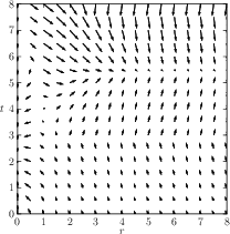
Fig. 1a: An exemplary vector field \( \nabla Z \) (eq: 2.2) representing the selective pressure on an individual as part of a finite population with the occurrence of mutants respectively.
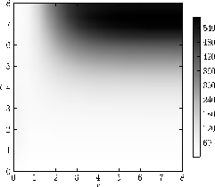
Fig. 1b: The individual fitness \( Z_i \) (eq: 2.1) in a homogeneous population without the occurrence of mutants.
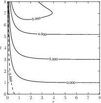
Fig. 1c: The qualitative behaviour of \( D(r)Q(I) \) in homogeneous resident populations as described in the derivation from (eq: 2.3) with values \( \leq 0 \) representing an increasing product with signal strength \( r \).
Figure 1: The different elements of evolutionary dynamics in the co-evolution of aposematism in finite populations. Parameters as in Figure 2a
The fitness of an individual is described by the payoff function \( Z_i \) (eq:2.1) and depends on its strategy \( (r_i, t_i) \) and on the composition of the population due to the generalisation of aversive information based on similarity. We consider invasion of a mutant group into a monomorphic resident population, i.e. all members of the resident population play an identical strategy. We will refer to the resident population with subscript \( 1 \) and to the mutants with subscript \( 2 \). Mutants can differ from residents in either of the two strategy components, and we consider the selective pressure in two different directions, one in each component. In each component we consider the payoff of mutants of different types \( x_2 \) against the resident population \( x_1 \), indicated by the payoff function \( Z(x_2,x_1) \). The selective pressure is defined by the derivative of the payoff function \( Z \) with respect to \( x_2 \) (strictly this derivative does not exist in the direction of \( r \) but the expression below is still meaningful as we discuss in Section 3.2), which is visualised as a gradient \( \nabla Z \) over a grid of points using a numerical 5 point stencil approximation of each partial derivative separately with \( h=1e-5 \) as follows: \[ \partial Z = \frac{-Z(x_1+2h,x_1) + 8Z(x_1+h,x_1) -8Z(x_1-h,x_1) + Z(x_1-2h,x_1)}{12h} ~~. ~~~~(2.2) \]
The population composition is defined by the values of the population size ( \( N \) ) and the mutant group fraction ( \( a \) ). The final visualisation shows the gradient of the payoff function \( \nabla Z \) as a vector field (Fig. 1a) representing the selective pressure, the fitness value of an individual in a homogeneous population in the background as a heat map (Fig.1b), and the behaviour of \( D(r)Q(I) \) as a contour plot (Fig. 1c). The product \( DQ \) can in principle increase, decrease or remain constant according to the choice of functions. It has been discussed that biologically meaningful functions should result in an increasing or only slowly decreasing product \( DQ \) with increasing signal strength \( r \) in homogeneous resident populations [Broom 2006]. Therefore, we require \( dDQ/dD > 0 \) with \( DQ=D(exp(-AD) + q_{min}) \) and from \[ \frac{d}{dD} DQ = \exp (-AD) - AD \exp (-AD) + q_{min} ~~~~(2.3) \] we have \( A<(1+q_{min}\exp(AD))/D \) where \( A=Nq_0H(t)/\epsilon \).
Corresponding to this derivation the contour plot in Figure 1c shows the values of \( A-(1+q_{min}\exp(AD))/D \) with values \( \leq 0 \) the product being increasing with signal strength \( r \).
Drift
In finite, and especially in small, populations, random sampling can result in a change of allele frequency [Masel 2011]. Consequently, natural selection is not the only force acting on populations and unfavourable mutations can take over entire populations. Therefore, the extent of drift needs to be considered in the evaluation of stability. The probability \( x_2 \) of a group of mutants ( \( a_n = aN \) ) invading a population is termed the fixation probability. The evolution of the population is modelled by a version of the Moran process [Moran 1962], which is the classical way to model the evolution of finite populations. The Moran process is a Markov process where the state of the population (in our case denoted by the number of mutants) changes according to a transition matrix, and each change represents the replacement of an individual by one of another type.
The determinant transition probabilities \( p_{i\rightarrow i+1} \) and \( p_{i\rightarrow i-1} \) that form the matrix are a combination of the chance of random selection and relative fitness \( w_F = F_2/F_1 \). As our model incorporates secondary defence, the transition probabilities are extended by the corresponding mortality \( w_K \) as defined in (eq: 2.4): \[ w_K = D(r)Q(I)K(t)~~.~~~~(2.4) \]
The final transition probabilities are a combination of random death and fitness related birth as presented in (eq: 2.5): \[ \begin{split} p_{i\rightarrow i-1} &= \frac{N-i}{w_F i + N-i} ~ \frac{i}{N} w_{K_2} , \\ p_{i\rightarrow i+1} &= \underbrace{\frac{w_F i}{w_F i +N-i}}_{birth} ~ \underbrace{\frac{N-i}{N} w_{K_1}}_{death}~~. \end{split}~~~~(2.5) \] Thus for the mutant to increase in number ( \( p_{i\rightarrow i+1} \) ) a resident individual has to encounter a predator ( \( ({N-i})/{N} \) ) and has to be killed ( \( w_{K_1} \) ) first. Secondly, it has to be replaced by a mutant according to the mutants relative fitness in the population ( \( ({w_F i})/({w_F i +N-i}) \) ).
For a group of mutants the fixation probability is given by the closed form of the transition matrix (eq: 2.6) [Weibull 1997, Nowak 2006]: \[ x_2 = \frac{1+\sum_{j=1}^{a_n-1} \prod_{k=1}^j \gamma_k}{1+\sum_{j=1}^{N-1} \prod_{k=1}^j \gamma_k} \quad with \quad \gamma_i = \frac{p_{i\rightarrow i-1}}{p_{i\rightarrow i+1}} ~~.~~~~(2.6) \]
To reflect the non-constant selection of the model, the relative fitness \( w_F \) and the mortalities \( \( w_K \) are recalculated on each step based on the changed population composition. The strategy of the mutants is chosen along the derivative of the payoff function (eq:2.7), that is, in the direction of strongest selection, to represent the toughest opponent possible with the highest fixation probability as follows: \[ \binom{r_2}{t_2} = \binom{r_1}{t_1} + h \frac{\nabla Z}{\Vert \nabla Z\Vert} ~~,~~~~(2.7) \] with \( h=1e-5 \). The final visualisations in Figure 2 show the diversion from neutral drift as a log score \( \log_{10}(Nx_2/a_n)/h \), with a score of zero occurring when \( x_{2}=a_n/N \), indicating equal fitness between mutants and residents and so full dominance of neutral drift over selective pressure. The fixation probability \( x_2 \) is only approximately linear in \( h \) for a small range of values because of the trade-off between detection probability and predator generalisation. Note that this means that the drift score too is only independent of \( h \) over small ranges.
For infinite populations a resident strategy which is fitter than any mutant strategy within a population composed of a mixture of the resident and mutant strategies, where the frequency of the mutants in the population is sufficiently small, can resist invasion from all such mutants, and is termed an Evolutionarily Stable Strategy (ESS). The spatial structure of the population can be considered by allowing the fraction of mutants in the local area to be a significant proportion of the population, even when their overal proportion is small, and this approach was taken in the previous models of [Broom 2006 and 2008] as well as in this paper. The definition of an ESS in a finite population requires an extra condition: in addition to the equivalent of the above condition (that the fitness of a single mutant within a population of residents is strictly less than that of the residents), we need the fixation probability of a single mutant to be less than \( 1/N \) [Taylor 2004, Nowak 2006]. For our model we consider an invading group of size \( a_{n} = aN \), and we thus adapt this definition accordingly: in order to consider the fitness of mutant and resident individuals within such a population mixture, we compare the fixation probability of the mutant group with the corresponding neutral probability of \( x_{2} =a_{n}/N = a \).
We note that in our model the two conditions above actually reduce to one (as is often the case), since the aversive Information function increases with the increasing number of mutants, so if a mutant is fitter than the resident population when introduced as a small proportion of the population it will still be fitter when in a larger proportion, so the fixation probability condition is always satisfied when the fitness condition is.
Results
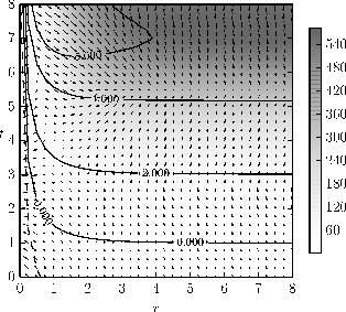
Figure 2-a1: Visualisation of the fitness landscape indicating the selective pressure on the population as described in Section 2.1 and detailed in Figure 1.
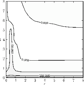
Figure 2-a2: Visualisation of drift as introduced in Section 2.2. The plot utilizes 3 significant figures leading to a wide area of approximately neutral drift within the 0.000 boundaries.
Figure 2-a: Exemplary adaptive dynamics of positive correlation for a simulation with the parameters: \( n = 500 \), \( \epsilon= 500 \), \( a_n = 200 \), \( v_0 = 1 \), \( d_0 = 1 \), \( t_c = 0 \), \( q_0 = 1 \), \( q_{min}=1e-3 \) , \( k_0 = 5 \), \( f_0 = 0.5 \).
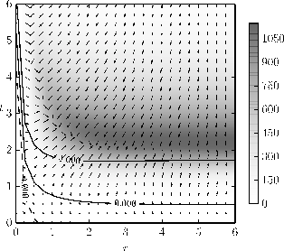
Figure 2-b1: Visualisation of the fitness landscape indicating the selective pressure on the population as described in Section 2.1 and detailed in Figure 1.
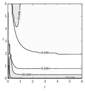
Figure 2-b2: Visualisation of drift as introduced in Section 2.2. The plot utilizes 3 significant figures leading to a wide area of approximately neutral drift within the 0.000 boundaries.
Figure 2-b:Exemplary adaptive dynamics of negative correlation for a simulation with the parameters: \( n = 500 \), \( \epsilon= 500 \), \( a_n = 250 \), \( v_0 = 10 \), \( d_0 = 1 \), \( t_c = 0 \), \( q_0 = 2 \), \( q_{min}=1e-3 \), \( k_0 = 5 \), \( f_0 = 1 \).
Figure 2: Results of the co-evolution of aposematism in finite populations including the influence of drift.
As natural selection acts on the individual level, in infinite populations an evolutionary stable solution (ESS) cannot be beaten by invaders (Appendix A) [Christiansen 1991]. However, reducing population size quickly increases the effect of drift [Whitlock 2000] which can destabilise populations. Using the functions presented in Table 2, the strategy dynamics were analysed regarding the co-evolution of \( r \) and \( t \) and the stability of strategies. Recall from Section 2.2 the conditions for a strategy to be an ESS in a finite population, and in particular that for our model we only need to consider a comparison of the fitnesses of resident and mutant strategies. Figure 2 shows two representative simulations. In general, the proportion of mutants needs to be relatively high for aposematism to evolve in small populations and the results will be discussed for each parameter respectively as follows.
Optimal Toxicity
The original model [Broom 2006 and 2008] predicted that the optimal toxicity \( t_{opt} \) will be an increasing function of \( r \) (Appendix A) and an exemplary simulation is presented in Figure 2a.
Additionally, Figure 2b shows the possibility of negative correlation between signal strength and level of defence. Firstly, we note that increasing \( t \) in equation (eq:A.3) in Appendix A also increases the product \( I_1Q'/Q \) so that scenarios with strong aversiveness \( H(t) \) are possible where the optimal toxicity is a decreasing function of \( r \) instead. That the aversiveness and its influence on the extent of learning can reverse the correlation between signal strength and level of defence represents a new insight for this model. Secondly, if the sizes of the gradients discussed in Appendix A are reversed, the optimal toxicity will be a decreasing function of \( r \) as the cost on fitness restricts investments into secondary defence.
This reflects two concepts: on the one hand, the signal correlates with the amount of secondary defence as the disadvantage of more conspicuous signals needs to be compensated for by better secondary defence. On the other hand, a clearer signal leads to more efficient aversive learning so that the investment into secondary defence can be lowered. The original claim in [Broom 2006] that the ESS value of \( t_1 \) , \( t_{opt} \), is increasing with that of \( r_1 \), \( r_{opt} \), if \( I_1>0 \), \( V(I_1) = -I_1Q'/Q \) is increasing with positive \( I_1 \) (eq:A.4) at \( r_{opt} \), and that \( D(r)Q(I_1) \) is an increasing function of \( r_1 \), can be violated by having a steep aversiveness function \( H(t) \). This allows a new type of solution for steep aversive information functions \( I_1 \) which depends on the scaling factor \( \epsilon \) and the aversiveness \( H(t) \).
Figure 2 also shows that if \( I_1 \) (eq:A.4) is not increasing sufficiently with large values of \( r_1 \), \( lim_{r_1 \rightarrow \infty} I_1Q'/Q = C \), the optimal toxicity levels out and is the solution to Equation (eq:3.1): all constant terms are positive, except \( C \) which is negative. For \( t_1>t_c \) the expression on the right decreases with \( t_1 \). For \( t_1 \) just bigger than \( t_c \) it is clearly positive, after which it is decreasing, and in the limit as \( t_1 \) tends to infinity it is negative. There is thus exactly one root in \( (t_c,\infty) \) which is \( t_{opt} \). \[ -f_0 + \frac{k_0}{1+k_0t_1} - \frac{aC}{t_1-t_c} = 0 ~~~~(3.1) \]
Aposematic signals
As discussed in [Broom 2006] and in the Appendix it is easier for mutants with weaker signals to invade a population and in infinite populations it is therefore sufficient to show that the left sided derivative of \( Z \) (eq:2.1) is positive for mutants with weaker signals \( r_2 < r_1 \). Through the introduction of drift, this argumentation is no longer valid. A sufficient condition for the existence of aposematic signals in finite populations remains that the left sided derivative of \( Z \) (eq: 2.1) is positive for mutants with weaker signals. The group size of mutants \( a \) describes the tradeoff between the influence of \( D'/D \) and \( S'(0) \). In the case of predators which are highly able to distinguish between individuals ( \( S'(0) \ll -1 \) ), the evolution of aposematism from crypsis requires \( a \) to be large, as mutants do not benefit from a predator's generalisation between residents and mutants (eq:A5b). </r_{1} \).>
With the focus on stability in finite populations, we must consider invasion by mutants with both higher and lower values of \( r_2 \). As we saw in Section 2.2, in our model the mutant that is the fittest when introduced at small frequency also has the highest fixation probability. Thus the key question is whether mutants with higher or lower values of \( r_2 \) are the fitter, and thus even when the left and right derivatives are different, the expression in Equation (eq:2.2) shows the pressure in the population due to drift. We would obtain a simple point solution where Equation (2.2) is equal to zero, provided that there is a compatible \( t_{opt} \). The condition that the right sided derivative of \( Z \) (eq:A6b) is negative for mutants with stronger signals is generally difficult to satisfy: as a group of mutants usually benefits in an aposematic population from the generalisation of aversive information, most solutions will be unstable in \( r \). Therefore, there is theoretically no stable level of signalling. However, the dominance of drift can create a pseudo-stability which has similar characteristics to the infinite amount of stable solutions with \( r_1>R \) as predicted for infinite populations in the Appendix. Here there is a range of different values of \( r_1 \) and \( t_1 \) which gives an area of stability rather than just a line: the extremely flat fitness landscape leads to a region where drift is approximately neutral to 3 decimal places (Figure 2).
With regard to the cryptic solution, it is always stable if the predator is not deterred by weak warning flags resulting in \( Q=1 \) and \( Q'=0 \). This is the case in the model presented as a consequence of the functional form of \( Q \) in Table 2.
Minimal attack probability
As discussed earlier, the introduction of a minimal attack probability \( q_{min} \) in equation \( Q \) in Table 2 avoids the problem of immortality in the model. There exist two options to introduce a minimal attack probability:
- On the one hand, the attack probability function \( Q \) can be shifted by \( q_{min} \) resulting in \( Q(I) = \min (1,\exp(-q_0 I) + q_{min}) \).
- A second possibility would be for the minimal attack probability to be realised using a simple cut-off value: \( Q(I) = mid (1,q_{min},\exp(-q_0 I)) \). The cut-off would result in \( Q'=0 \) for sufficiently low values of \( Q \), which requires stronger optimal secondary defence considering Equation (3.1).
Option 1, using a shifted function \( Q \), is the favourable choice of our model as we think results are more realistic (the results of option 2 are not presented) and allows the interpretation as a source of secondary cause of death as we discuss as follows: for high values of \( (r_1,t_1) \) the fitness function is extremely flat and changes in the parameters \( (r,t) \) have barely any effect on the payoff which is clearly dominated by almost neutral drift. This results in \( Q \) being effectively independent of \( (r,t) \) and \( q_{min} \) being the dominant influence. This means that the minimal attack probability behaves similar to the introduction of a secondary cause of death \( \lambda \). Even though this model is simplified assuming \( \lambda=0 \) (eq:A2) it is able to reproduce the effects of secondary causes of death.
Conclusions
This paper introduces a more flexible methodology for assessing evolutionary stability in previous game theoretical models of the co-evolution of aposematic signalling and secondary defence [Broom 2006 and 2008]. Our main conclusions are:
- the number of mutants needs to be relatively high (e.g. within a locality of the population) for aposematism to evolve in small populations,
- drift is an important force acting on real population systems and increases inter-population diversification of aposematic solutions,
- in terms of evolutionary stability drift results in a region comparable to an evolutionarily stable set (ESSet), where strategies can change within the region due to approximately neutral drift, but resist invasion from outside,
- anti-apostatic selection (selection against rare prey types) prevents intra-population dishonesty of the aposematic display (automimicry as well as continuous variation in toxicity), and
- enhanced predator aversion learning reduces the level of aversive defence investment through the compensation of more conspicuous displays.
In previous models of the co-evolution of aposematic signalling and defence [Broom 2006 and 2008] the conditions for the evolutionary stability of a signal and associated level of defence were found for a model assuming a large (effectively infinite) population. A feature of the model was that there was an infinite set of evolutionarily stable strategies (ESS) in many cases, where for a given level of signal there was a unique level of defence, but as long as the whole population displayed the same signal it was stable against invasion by any other strategy. In particular this infinite set consisted of a continuum (a line) of ESSs, so for any ESS a small mutation could be to another ESS as a potential invader. Thus it was of particular interest to consider finite populations, and consequently the effect of drift, and whether the strategies which were ESSs in the original model could still be considered stable.
Hence, we shall elaborate on how the introduction of drift as an additional evolutionary force in finite populations acts on the resident population. Drift cannot be neglected when the population size is relatively small and the payoff function is relatively flat, as in the original models. As a side effect of the flat gradient of the payoff function almost neutral drift dominates for values of high secondary defence and strong signal strength. Even though a distinct aposematic solution may exist, populations hardly converge towards them as drift dominates selective pressure. Notably in the case of small population size, the diversity of aposematic solutions extends from the previously predicted line to a wider plane-like parameter range (Figure 2). With regard to stability this result can be interpreted as a finite population version of the idea of an evolutionarily stable set, where strategies can change within the region due to drift, but resist invasion from outside. The widespread variation of secondary defence and aposematic displays has been discussed in [Speed 2010] as a consequence of frequency-dependent intra-population cheating in an ecological model in which prey acquires its anti-predatory defences from the environment, e.g. from a food source. In our co-evolutionary model the inter-population diversification is a consequence of drift which is an interesting result: intra-population cheating (or automimicry) is problematic in the context of evolutionary stability as it undermines the effectiveness of the signal since cheating appears to be at a selective advantage [Jones 2013]. Drift instead allows a wide diversity of inter-population aposematic solutions without the introduction of destabilising cheating or automimicry on the intra-population level.
On the other hand, the stability of aposematism is tightly bound to anti-apostatic selection: even though the diversity of stable inter-population aposematic solutions is high, a stable aposematic population needs to look alike or the level of aversive information suffers and aposematism loses its advantage (eq:A5b). The required degree of uniformity depends upon the predator's ability to distinguish different prey individuals ( \( v_0 \) ). The condition of close resemblance holds if mutations are mostly silent without effects on the phenotype and the mutation rate is reasonably low.
In addition to the solutions predicted from the earlier models of [Broom 2006 and 2008], we observed a new set of possible solutions with negative correlation between secondary defence and signal strength (Figure 2b). For this solution to appear, the aversiveness of secondary defence needs to be rapidly increasing or the predator needs to be very sensitive towards aversive information. Under these circumstances, increasing conspicuousness improves prey distinction and stimulates aversive learning to such a degree that necessary investments into secondary defence can be lowered. This result is contrary to the decreasing aposematic display with increasing toxicity as consequence of aposematic display and investment into toxicity competing for a common resource in [Blount 2009, Lee 2011]. In our model the accelerated learning process of strong aversion is the reason of the negative correlation and allows lower levels of toxicity with increasing conspicuousness. See [Speed 2007] for another example of this phenomenon as a result of specific marginal costs using Gompertz functions rather than aversive learning.
Generally, the frequency of mutants has to be relatively high for aposematism to evolve in small populations. This may be seen as requiring a component of kin selection or the invasion of a rivalling population into a locality.
Furthermore, the predatory risk of death needs to dominate other risks of death for aposematic solutions to emerge. As an unbounded payoff function has the side effect of unrealistic immortality the attack probability needs to have a minimal value of \( q_{min} \). This makes additional risks of death redundant as they can be considered as part of \( q_{min} \) as discussed earlier.
Finally, the cryptic solution is always stable if the predator is not deterred by small diversions from full crypsis. This seems like a reasonable conclusion and for questions related to the possibility of overcoming the stability of crypsis this paper refers to models of the initial emergence of aposematism describing mechanisms such as dietary conservatism, a shifted peak of the aversive information function, the opportunity cost of crypsis, and specific properties of the predator's perception or cognitive processes [Mappes 2005, Mapes 2005b, Speed 2005, Lee 2011].
Future work will require a more sophisticated description of aversive learning moving from the equilibrium of educated predators to the original considerations of uneducated predators. The introduced methodology will make it possible to answer questions related to the transmission of learning, i.e. where/how predators learning can evolve, the configuration of warning displays and how context and environment affect aversiveness and learning. Reinforcement learning will be used to look into conditions of special cases such as heterogeneity and mimicry, which cannot be explained by bare co-evolution of warning displays and secondary defences.
Appendix A: The model of co-evolution.
| Symbol | Meaning |
|---|---|
| \( r \) | the conspicuousness of an aposematic signal |
| \( t \) | the level of toxicity of secondary defences |
| \( K(t) \) | the probability that an individual of toxicity t is killed in an attack |
| \( H(t) \) | the aversiveness of an individual of toxicity t |
| \( S(x) \) | the similarity function of individuals differing in appearance by \( x \) with \( x=\vert r_1 - r_2\vert \) |
| \( I(r) \) | the level of aversive information of an individual |
| \( D(r) \) | the rate at which individuals of conspicuousness \( r \) are detected |
| \( Q(I) \) | the probability that a predator will attack an individual associated with a level of aversive information \( I \) |
| \( a \) | the fraction of mutants in the population |
| \( t_c \) | the level of toxicity which becomes aversive, hence for which \( H(t_c ) = 0 \) |
Table 3: Exemplary functions as introduced in [Broom 2006 and 2008]
In [Broom 2006] a game theoretic model of prey-predator interaction was introduced to describe the co-evolution of secondary defence and signalling. The model investigates the general mechanisms of aposematism rather than specific species or environments, assuming general function shapes. Building on that, the model was further developed in [Broom 2008] using exemplary and plausible functions (Table 3) to demonstrate the solutions predicted from [Broom 2006].
The model from [Broom 2008] considers a single population of prey individuals where individuals \( i \) are described by two parameters \( (r_i, t_i) \).
The parameter \( t \) reflects the individual investment into secondary defence. This secondary defence is not observable by the predator and could be unpalatable toxins, for example. The expression of secondary defence comes with a cost of decreasing fecundity \( F(t) \). On the contrary, secondary defence is advantageous in surviving an attack, reducing the chance of being killed \( K(t) \).
The parameter \( r \) describes the conspicuousness of an aposematic signal, with \( r=0 \) referring to maximal crypsis. The quality of signalling is associated with an unfavourable higher rate at which individuals are detected by predators \( D(r) \). In contrast, conspicuousness of an aposematic signal is beneficial in combination with secondary defences by increasing the predator's level of aversive information regarding an individual.
Unlike the model of [Leimar 1986] where naïve predators learn to avoid unpalatable prey types, the model of [Broom 2006] is assumed to be in equilibrium: population sizes are constant and predators are educated and have full knowledge of the population’s aversiveness and signalling strategies. This knowledge is expressed in a level of aversive information ( I ) about individuals which depends upon the appearance of the individual in question, and the properties of the population of prey individuals.
A prey individual contributes to the level of aversiveness about others through a combination of three factors. Firstly the likelihood of it being encountered, which is proportional to the detection probability \( D(r) \) described above. Secondly the aversive effect of its consumption, which depends upon its value of \( t \) through the function \( H(t) \), which is increasing with \( t \). There is a critical value of defence \( t_{c} \) for which \( H(t_{c})=0 \); this corresponds to levels of defence above this being aversive, and levels below this being actually beneficial, encouraging the consumption of more prey of this type.
Finally, this individual will affect the response of the predator to others only if it is sufficiently similar to them, which is indicated by the similarity function \( S(x) \), where \( x=|r-r_{j}| \) is the difference between the \( r \) value ( \( r_{j} \) ) of the above individual and that of any given targeted individual. If \( x \) is large, then the two are very different and the similarity function is very small. For \( x=0 \) they are identical, and the similarity function is set to equal 1. The peaked form of the similarity function (where the function is differentiable w.r.t \( r \) everywhere but at the peak, where the left-derivative and right-derivative are different) is characteristic of this model and responsible for the resulting broad range of alternate ESS.
The information from a single population individual with parameters \( (r_{j}, t_{j}) \) about our focal individual with parameters \( (r_{i}, t_{i}) \) is thus proportional to \( D(r_{j})H(t_{j})S(|r_{i}-r_{j}|) \). The total aversive information from the population is the sum of this over all individuals (in the original work this was multiplied by the ratio of prey individuals \( N \) to predators \( n \), but this is simply a scaling factor), giving \[ I_{i}=\sum_{j=1, j \neq i}^{N}D(r_{j})H(t_{j})S(|r_{i}-r_{j}|) ~~. ~~~~(A1) \]
The predator then uses the information about individual \( i \) to decide whether to attack it if it is encountered, choosing the attack probability \( Q(I) \), which is decreasing in \( I \), based on the amount of aversive information \( I_i \).
The payoff to an individual, which is simply the ratio of its fecundity \( F(t_{i}) \) and its rate of being killed, is described as follows: \[ Z_i = \frac{F(t_i)}{D(r_i)Q(I_i)K(t_i) + \lambda} ~~. ~~~~(A2) \]
The original model adds a constant \( \lambda \) to the denominator to represent death due to events other than predation, but in some of the analysis in that paper (and in this one) this term is set to zero.
The evolution of secondary defences is promoted by an increased inclusive fitness through both the greater chances of escape of individuals, and the reduction of the likelihood that educated predators re-attack prey individuals or their relatives in the future. Modelling the evolution of signalling and defence using kin grouping was introduced in [Leimar 1986], destabilising crypsis in favour of aposematism. The parameter \( a \) in the model of [Broom 2006] describes the initial protection of mutants from predation: mutants occur in groups with local proportion \( a \) either as a consequence of first appearing in a self-contained locality or through invasion.
The main findings of the underlying model of [Broom 2006] were:
- Crypsis can be destabilised without the assumption of a naïve tendency of avoiding suspicious prey individuals or the usage of a peak-shifted aversiveness towards more suspicious individuals by co-evolution.
- The strength of aposematic displays is a reliable indicator of the strength of defence, that is, the correlation between the two is positive.
- If the conditions support the emergence of aposematism there are multiple stable solutions laying on an increasing line \( t_{opt}(r) \) . Hence, the diversity of different solutions for secondary defence and warning displays is a consequence of the underlying co-evolution.
- Aposematism is not a necessary condition for optimality of highly defended prey populations and stable cryptic populations can possess aversive levels of defence.
- There are conditions which interfere with anti-apostatic selection and allow diversity of appearance in poorly defended prey individuals.
Optimal Toxicity
As for the question of optimal investment into costly defence, the level of secondary defence is not observable by the predator and has no effect on the generalisation of aversiveness. The optimal toxicity of this model \( t_{opt} \), where \( \partial Z / \partial t = 0 \) the derivative of \( Z \) w.r.t \( t \) is 0 at \( t=t_{opt} \) in a population which plays \( t_{opt} \), is given by \[ g_1 = \frac{F'}{F} - \frac{K'}{K} - aI_1\frac{Q'}{Q}\frac{H'}{H} = 0, ~~~~(A3) \]
where \( F' \) represents the derivative of the fecundity function (and similarly for other functions), and each function is evaluated at \( t=t_{opt} \) and a specifc value of \( r \) (for a given \( r \)-value, \( t_{opt} \) will be different).
We refer to the resident population with subscript \( 1 \) and to the mutants with subscript \( 2 \). Following the definition of function \( I \) in [Broom 2008], the level of aversive information for the resident population is given as follows: \[ I_1=((1-a)D(r_1)H(t_1)+aD(r_2)H(t_2)S(x)) ~~. ~~~~(A4) \]
If the product \( I_1Q'/Q \) is decreasing with \( r_1 \), equation (eq:A3) increases with \( r_1 \). This increase is compensated for by a variation of the optimal toxicity. If the absolute gradient \( \vert d/dt(K'/K)\vert \) is greater than \( \vert d/dt(F'/F)\vert \) the benefits of secondary defence outweigh the cost on the fitness and the optimal toxicity will be an increasing function of \( r_1 \).
Aposematic signals
Regarding aposematic signals, the predator generalises aversive information between the resident population and mutants based on their similarity in appearance described by the similarity function \( S(x) \). Mutant groups can potentially invade a resident population from two directions. Using the terminology of Broom et al. 2006, the conditions for resisting mutant invasion are a composition of the effects of recollection on the amount of aversive information \[ g_2 = D'/D + aI_1Q'D'/QD ~~~~(A5a) \] and the effects of generalisation \[ g_3 = (1-a)I_1Q'S'(0)/Q ~~~~(A5b) \]
Due to the peaked shape of the similarity function \( S(x) \), these conditions are different for mutants with higher and lower values of \( r_2 \) than the population. For \( r_2 <r_1 \) they depend on the left derivative of \( Z \): \[ \frac{\partial Z_{l}(r_1,r_{2})}{\partial r} = -g_2 + g_3 \quad for \quad r_2 < r_1 ~~~~(A6a) \] which must be positive for stability, and for \( r_2>r_1 \) the right derivative of \( Z \) \[ \frac{\partial Z_{r}(r_1,r_{2})}{\partial r}= -g_2 - g_3 \quad for \quad r_2 > r_1 ~~~~(A6b) \] which must be negative for stability.
This makes it easier for mutants with weaker signals to invade a population. Therefore, it is sufficient for stability of aposematic signals in infinite populations to show that (eq:A5a) is positive for mutants with weaker signals \( r_2 < r_1 \).
With regard to cryptic solutions ( \( r_1=0 \) ), a population can only be invaded by more conspicuous mutants ( \( r_2 > r_1 \) ). The cryptic solution is stable if \( -g_2 - g_3 < 0 \). From this follows:
- There is always a cryptic stable solution if there is no investment into secondary defence which occurs if \( g_1(r_1=0, t_1=0)<0 \).
- In the case of an investment into secondary defence a cryptic solution is only stable if this investment is aversive causing \( I_1>0 \), \( a \) is sufficiently small (below some critical value) and the predator is able to sufficiently distinguish between the resident population and mutants.