I used three methods on simulated data-sets to evaluate their performance. The simplest approach is by the edgeR method which assumes a linear relation of mean and dispersion. The DESeq method extends this approach to an non-linear data-driven dependency. The baySeq method uses general Bayesian methods to estimate posterior probabilities.
All three methods counteract the over-dispersion owned by the biological variance with negative-binomial distributions. In the introduction, I give an overview of the over-dispersion problem and the different normalization methods used by the three methods.
Introduction
Next generation sequencing with its high throughput offers new experimental set-ups in gene expression studies. Thereby discrete counts of sequence tags are used to approximate the continuous nature of gene expression. This new technology raises questions on how to analyse this count data from high-throughput sequencing and the evaluation of expression differences in experimental set-ups. As with any measurement or comparison of measurements it is essential to know the variance of the data in order to reveal anything significant about the results. As it turns out, estimating the variance of sequence count data is a complex and challenging task.
Technical Variation
The systematic technical errors of cDNA library construction such as PCR amplification or RNA-ligase preferences lead to a strong bias towards certain small RNAs [Tian2010, Linsen2009]. But as this biases are systematic and reproducible deep sequencing is still suited for analysing relative expression differences. Sequencing a cDNA is a multinomial process which is approximated tag-wise by Poisson distributions where the chance of a tag being sequenced is exponentially distributed. The problem with the Poisson model is that it underestimates the effect of biological variability and only the variance of technical replicates follows the Poisson model perfectly. Because the sum of normalized square deviations distributes approximately as \(\chi^2\) if the \(\lambda\) is of reasonable size (\( \lambda > 5 \) is assumed) \[ \sum\frac{X_i - \lambda}{\lambda} \sim \chi^2 \] it can be used to test whether the difference between the counts is greater than expected between technical replicates.
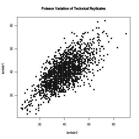 The variable variance of technical replicates.
The Fisher test is an exact version of the \(\chi^2\) test which calculates the significance of the deviation from the null hypothesis exactly, whereat the \( \chi^2 \) test is an asymptotic test which converges for large sample sizes. The Fisher test therefore provides better results for marginally represented sequence tags, but as with the \( \chi^2 \) approximation, the Fisher test only reveals the significance of technical replicates. For large counts the Normal distribution can be used as a good approximation of between replicate variability with \( \mu=\lambda \) and \( \sigma^2=\lambda \). \[ f_\lambda(x) \approx \frac{1}{\sqrt{2\pi\lambda}}\exp\left(-\frac{(x-\lambda)^2}{2\lambda}\right) \]
Over-dispersion
Even with microRNA expression profiles, for example, which are generally conserved and adequate bio-markers, the Poisson model underestimates the biological variance because the Poisson distribution is a one-parametric distribution with \( \mu=\sigma^2=\lambda \). \[ f_\lambda(x) = \frac{\lambda^x}{x!}e^{-\lambda} \] This results in greater sample variation than expected because the model is oversimplified. This is called over-dispersion and leads to an uncontrolled type-I error, which is the reason why z-scores and log-linear approaches classify almost every expression variation as highly significant. An advantage of deep sequencing in mircoRNA profiling is that it can capture transcriptome dynamics without sophisticated normalization methods in direct RNA sequencing approaches [Ozsolak2009]. To be able to compare deep sequencing results the counts need to be independent of the sequencing depth. Consequently, common normalization strategies are scaling to library or sub-library sizes and quantile normalization [Meyer2010]. At present, however, most experimental set-ups are non-direct and standard normalization methods are not sufficient to remove the bias and deal with the over-dispersion of the deep sequencing data.
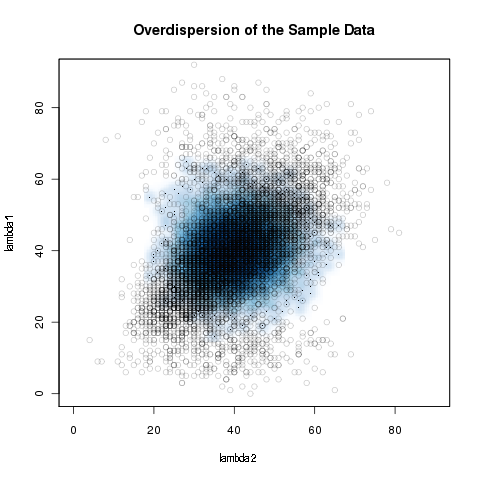 Overdispersion of the simulated sample data. The blue density represents the Poisson model.
TMM Data-Normalization
In case a small fraction of genes are highly over-represented within a cDNA library, the remaining genes in the library are under-sampled. To address this, Robinson et al. developed the trimmed mean of the M-values normalization method which is an empirical approach at respecting this bias by introducing an effective library size [Robinson2010]. Under the assumption that the majority of the genes are not differentially expressed, the gene-wise log-fold changes \( M_g \) and the absolute expression levels \( A_g \) are calculated
\[ M_g = \log_2 \frac{Y_{gj} / l_j}{Y_{gj'} / l_{j'}} \]
\[ A_g = \frac{1}{2} \log_2 \left( \frac{Y_{gj}}{l_j} * \frac{Y_{gj'}}{l_{j'}}\right) \]
where \( l \) is the library size represented by the total amount of reads, \( Y \) the corresponding counts of gene \( g \) in sample \( j \).
By default the list of \( M_g \) values is trimmed down by the 30\% most extreme values and the list of \( A_g \) values by 5\%. After trimming, a weighted average of \( M_g \) is calculated where the weight is the inverse of the approximated asymptotic variances using the delta method which estimates the variance of \( M_g \) across the libraries. This approach respects the lower variance of log-fold changes of larger read counts.
The final normalization factor for sample \( j \) ( \(f_j \) )is calculated as:
\[ f_j = \log_2(TMM_j^{(r)}) = \left( \sum_{g\in G^*} w^r_{gj}l^r_{gj} \right) * \left( \sum_{g\in G^*} w^r_{gj} \right)^{-1} \]
where \( r \) refers to the reference sample and \( G^* \) represents the trimmed set of genes with valid \( M_g \) and \( A_g \) values and the weight is given by:
\[ w^r_{gj} = \frac{l_j-Y_{gj}}{l_j Y_{gj}} + \frac{l_r -Y_{gr}}{l_r Y_{gr}} \]
Finally, the reference library is divided by \( \sqrt{f_k} \) and the non-reference libraries multiplied by \( \sqrt{f_k} \).
This procedure normalizes the sequence counts to the effective library size which is stable against few highly over-represented sequences due to trimming of the extreme values.
Negative-Binomial Distribution
To use statistical testing to obtain the significance of observed differences in read counts, an estimation of their variability throughout the dynamic range of low counting and highly over-expressed reads is needed. To avoid over-dispersion, it is proposed that negative binomial distributions are used, which can be derived from a Poisson distribution, where \( \lambda \) itself is a random variable following a Gamma distribution, which represents the sum of independent exponentially distributed random variables whereat the chance of a sequence tag being sequenced in a Poisson process is exponentially distributed. The NB distribution is a two parametric distribution, determined by mean and variance. However, usually the number of replicates is too small to estimate both parameters reliably for all the genes from the data.
Comparison of 3 different methods
edgeR The gold standard
One approach is the one by Robinson et al. which assumes that mean and variance are related with a single proportionality constant \( \phi \) \[ \sigma^2 = \mu + \phi\mu^2 \] where counts \( Y_{gij} \) - with \( Y \) are the counts of gene \( g \) under condition \( i \) replicate \( j \) - are modelled NB distributed as: \[ Y_{g,j:\rho(j)=\rho} \sim NB(l_j*p_{g,j:\rho(j)=\rho},\phi_g) \] where \( l_j \) is the library size represented by the total number of reads, and \( p_{g,j:\rho(j)=\rho} \) is the proportion of this sequenced gene. \( \phi_g \) is the over-dispersion representing the biological variation. With \( \phi_g=0 \) this model reduces to the original Poisson model and in this way, it separates biological from technical variation.
The library size is corrected using the TMM approach and the gene-wise variance is estimated at the maximum likelihood conditioned on the total count for that gene. The conditional likelihood approach produces unbiased estimates of the variance because it takes into account the loss of degrees of freedom in calculating the mean. For this approach equal library sizes are assumed which is not the case in the usual experimental set-ups. In this case an approximation approach is used which creates quantile-adjusted pseudo-data. Using an initialized value for the biological variance \( \phi \), a rate \( \lambda \) is estimated and by assuming that the data is given by an NB distribution with the mean \( m*\lambda \) - where the size parameter ( \( m \) ) is approximated by the geometric mean of the library sizes \( l_j \) - the observed percentiles are calculated [Robinson2008].
Using a linear interpolation of the percentiles, pseudo-data is calculated from an NB distribution \( NB(m*\lambda,\phi) \) following the given percentiles and will be approximately identically distributed for each gene. On this pseudo-data the variance \( \phi \) is calculated using the conditional likelihood approach which converges by iteration. This iteration reflects an empirical Bayes procedure, which is an iterative scheme to estimate the prior distribution from the data, to derive a mutual variance value by sharing information among genes.
The quantile adjustment leads to approximately identically distributed pseudo-data which offers exact testing using a modified Fisher’s exact test, where the hyper-geometric probabilities are replaced by the NB distribution. This leads to a two-sided p-value, which is the sum of the condition totals that are less likely than those observed. But because the pseudo-data is an approximation of identical distributed data, the p-value is also only an approximation, even the test is exact.
DESeq error modelling to achieve statistical power
The DESeq method extends the edgeR approach of the single parameter \( \phi \) relationship of mean and variance to a more general data-driven relationship [Anders2010]. But otherwise it also assumes a NB distribution.
\[ Y_g \sim NB(\mu_{gj},\sigma^2_{gj}) \]
where the mean \( \mu \) of a gene \( g \) in sample \( j \) is \( \mu_{gj}=l_j*q_{gj} \) and \( l_j \) is the library size and \( q_{gj} \) a condition dependent per-gene value which can be interpreted as a rate.
The variance is a combination of two terms:
\[ \sigma^2_{gj} = \underbrace{\mu_{gj}}_{\mbox{shot noise}} + \underbrace{l_j^2*v_\rho(q_{g,j})}_{\mbox{raw variance}} \]
where the raw variance is a smooth function \( v_\rho \) of the per-gene condition dependent rate factor.
Looking closer the model has the following properties:
- The noise term is dominant for low count values, which can be improved by deeper sequencing.
- The shot noise term is fairly unimportant for high count values where the raw variance dominates because the biological noise exceeds the technical shot noise term by many orders of magnitude. Improvement can only be achieved by replicates.
The library size is estimated by: \[ \hat{l}_j = \underset{g}{\mbox{median}} \ \left( Y_{gj} \right) * \left( \left( \prod_{v=1}^J k_{gv} \right) ^{\frac{1}{J}} \right) ^{-1} \] where \(Y \) is the counts of gene \( g \) in sample \( j \) and \( J \) the total amount of samples. The denominator can be interpreted as a pseudo-reference derived from the geometric mean across samples. Finally, the estimated library size is the median of the ratios of the gene counts to the pseudo-reference. According to [Anders and Huber 2010] this approach is more robust than the sums \( \sum_g k_{gj} \) in case of few highly abundant counts.
The gene and condition specific expression rate is estimated as: \[ \hat{q}_{g,\rho} = \frac{1}{J_\rho} \sum_{j:\rho(j)=\rho} \frac{Y_{gj}} {\hat{l}_j} \] where \( \rho \) is the condition and \( j:\rho(j)=\rho \) the specific condition of the sample \( j \) and \( J_\rho \) the total amount of replicates of the condition \( \rho \). This estimator is the average counts of all samples corresponding to condition \( \rho \) normalized by the estimated library size \( \hat{l}_j \).
Given these equations it leads to unbiased estimators of the raw-variance with: \[ \hat{v}_{g,\rho} = \underbrace{ \frac{1}{l_\rho-1} \sum_{j:\rho(j)=\rho} \left( \frac{Y_{gj}} {\hat{l}_j} - \hat{q}_{j,\rho} \right) ^2}_{\mbox{normalized sample variance } \displaystyle{w_{g,\rho}}} - \underbrace{\frac{\hat{q}_{g,\rho}}{J_\rho}\sum_{j:\rho(j)=\rho}\frac{1}{\hat{l}_j}}_{\displaystyle{z_{g,\rho}}} \]
But the problem is that the normalized sample variances vary highly if the number of replicates is small, as is typically the case. Therefore, a local regression is used to obtain a smooth function of the sample variance \( w_\rho(q) \) based on the \( (\hat{q}_{g,\rho}, w_{g,\rho}) \) graph. The final raw-variance estimate is given by: \[ \hat{v}_\rho(\hat{q}_{g,j}) = w_\rho(\hat{q}_{g,j}) - z_{g,\rho} \]
Testing for differential expression
The test statistic is based on the null-hypothesis that the gene and condition-specific rate parameters for both conditions are the same and consists of the gene counts in each condition \( K_{iA}=\sum_{g,\rho(j)=A} Y_{gj} \) and the overall sum \( K_{gS} = K_{gA} + K_{gB} \) and is analogous to conditioned tests as Fisher's exact test. The underlying distribution is the NB distribution. Simulated data showed that an NB distribution characterised by the mean and variance estimates shows no uniform p-values on non-differentially expressed data, which are also too small in the case of low replicate numbers. Therefore the NB distribution is re-parametrized to be specified by mean and the SCV \( \frac{\sigma^2}{\mu^2} \).
Testing without replicates
Having no replicates for one or even both conditions limits strongly the reliability of the analysis but is m¬aybe useful for exploration and hypothesis designment. In the case where replicates are only available for one condition, it can be assumed that the variance estimate also hold true for the unreplicated one. If there is no replicate available for both conditions, it can be assumed that most of the tags are not affected by the different conditions. By treating both samples as replicates a minority of differentially expressed genes will show up as outliers. In the final gamma-family fit this has almost no impact because the Gamma distribution \( \Gamma(k,\theta) \) for only the two replicates \( (J=2) \) and ( \( k=\frac{J-1}{2} \) ) has strong tale. But the overall effect is a overestimation of the variance which makes the approach conservative.
baySeq empirical Bayesian method
This approach uses general Bayesian methods to estimate posterior probabilities for defined models [Hardcastle2010]. The definition of models is done by the user and can be complex. In the most general pairwise comparison of two conditions \( A,B \) with replicates, it is assumed that at least some genes are not affected by the different conditions and the corresponding model of none differential expression would be \( \{A_1,A_2,B_1,B_2\} \) and the model for differential expression would be \( \{A_1,A_2\} \ \{B_1,B_2\} \). The data-set is defined as \( D_g = \{ (Y_{g,1}, Y_{g,2} \dots),(l_1, l_2 \dots)\} \) with the counts \( Y \) of gene \( g \) with the corresponding library sizes \( l \). Considering some model \( M \) the quantity of interest is the posterior probability of the model given the data-set: \[ P(M|D_g) = \frac{P(D_g|M) P(M)}{P(D_g)} \]
Calculating \( P(D_g|M) \)
Given a model \( M \) which is defined by a set \( \{E_1,E_2\dots E_q\} \) and the corresponding underlying distributions \( \{\theta_1,\theta_2\dots \theta_q\} \), a set \( K \) is defined as \( K=\{\theta_1\dots\} \). To calculate \( P(D_g|M) \) which is the probability of the data-set given a model \( M \), one approach is to use marginalisation to integrate over the sets of distributions which provides the unconditioned model. \[ P(D_g|M) = \int P(D_g|K,M) P(K|M) dK \] Under the assumption that the distributions \( \theta_q \) are independent with respect to \( q \) the dimension of the integral can be reduced: \[ P(D_g|M) = \prod_q \int \underbrace{P(D_{qg}|\theta_q)}_{\text{mixed Poisson dists}} \overbrace{P(\theta_q)}^{\text{Gamma dist. Poisson rates}} d\theta_q \] Based on the earlier discussion an NB distribution is used which is also know as the Gamma-Poisson-mixture distribution. The further approaches depend on equal library sizes, but library sizes are not equal. Instead of using the quantile-adjusted conditional maximum likelihood approach, an empirical Bayesian method is used where the prior distribution is estimated from the data. With this numerical method the real data can be retained and the library size is simply used as a scaling factor. The counts of a sample belonging to a set \( E_q \) have the mean \( \mu_ql_j \) and dispersion \( \phi_q \), so that the distributions are given by \( \theta(\mu_q,\phi_q) \). A approximation of \( P(D_g|M) \) can be derived from a set of values \( \Theta_q \) sampled from the distribution \( \theta_q \). This sampling is done by finding similar estimated dispersion factors (1) and means (2) of the sets \( E_q \) derived from count data belonging to the same sample \( E_q \). This is an empirically derived distribution on the set \( K \).
- The problem is to estimate a reliable dispersion: Because we do not know which genes belong to which model, a truly differential expressed gene tested in the model of no differential expression would lead to a strong over-estimated dispersion. The solution is an iterative quasi-likelihood method which initializes a mean-estimator based on the knowledge of replicates to converge the real dispersion of the data.
- The mean is derived by maximum likelihood: the mean which maximizes the NB distribution \( P(D_{qg},\phi_c,\mu_{qg}) \)
This will lead to the set \( \Theta_q=\{(\mu_{qg},\phi_c)\} \) so \( P(D_g|M) \) \) can be calculated.
Estimating \( P(M) \)
To calculate the prior probability of a model \( M \), an arbitrary initial value \( p \) is chosen as \( \hat{P}(M) \) in order to estimate the posterior probability \( P(M|D_g) \) by: \[ P(M|D_g) = \frac{P(D_g|M)\hat{P}(M)} {P(D_g|M)\hat{P}(M) + (1-P(D_g|M))*(1-\hat{P}(M))} \] Based on this new calculated posterior probability, it is possible to derive an improved estimation of the prior probability \( P(M) \) by: \[p' = \underset{g}{\mbox{mean}} \ P(M|D_g) \] By iteration the prior probability converges on the true value of \( P(M) \)
The marginal probability \( P(D_g) \)
The scaling factor \( P(D_g) \) can be determined by the sum over all the models, given their prior probability \( P(M) \) because there is only a finite set of models. \[ P(D_g) = \sum_i P(D_g|M_i)P(M_i) \]
Simulated Test-Data
To compare the performance of the three methods, I simulated data-sets of known composition. The test-samples consist of two samples each with two technical replicates. For each sample a library size \( (l) \) between \( 3*10^4 \) and \( 9*10^4 \) is sampled. The counts for each tag are calculated as follows:
| sample 1 | sample 2 | ||
|---|---|---|---|
| A1 | A2 | B1 | B2 |
| \( \lambda_{1,1}l_1 \) | \( \lambda_{1,2}l_1 \) | \( \lambda_{1,3}l_2 \) | \( \lambda_{1,4}l_2 \) |
| \( \lambda_{2,1}l_1 \) | \( \lambda_{2,2}l_1 \) | \( \lambda_{3,1}l_2 \) | \( \lambda_{3,2}l_2 \) |
The first line represents a non-differentially expressed tag and the second line represents a differentially expressed tag. In the case of non-differentially expressed tags, an expression rate is sampled from the black distribution ( \( \lambda_{1,n} \) ). The final expression rates ( \( \lambda_{1,1 \text{to} 4} \) ) are derived from the Poisson distribution characterized by the sampled expression rate. In the case of differentially expressed tags, the first expression rate ( \( \lambda_{2,n} \) ) is sampled from the black distribution and the second expression rate ( \( \lambda_{3,n} \) ) is sampled from the red distribution. The final expression rates are again derived from the Poisson distribution characterized by the sampled expression rates.
 Distribution of the expression rates of the simulated samples. The black bars represent the non-differentially expressed tags and the red bars the differentially expressed tags.
Results
The edgeR method which uses a linear variance fit in combination with a modified Fisher's Test shows the expected Type-I error of \( 0.05 \) due to the p-value cut-off. The local variance estimation of the DESeq method controls the Type-I Error and leads to no false positive in the non-differentially expressed sample.
| edgeR | DESeq | baySeq | ||||||
|---|---|---|---|---|---|---|---|---|
| diff=0 | diff=0.1 | diff=0.5 | diff=0 | diff=0.1 | diff=0.5 | diff=0 | diff=0.1 | diff=0.5 |
| FP=0.05 | TP=0.87 | TP=0.754 | FP=0 | TP=0.75 | TP=0.818 | FP=0.099 | TP=0.9 | TP=0.912 |
| FP=0.038 | FP=0.04 | FP=0.001 | FP=0.04 | FP=0.143 | FP=0.348 | |||
 Plot of the data sample with 0.1 differentially expressed tags. The mean is centred to the library size and the expression rates normalized.
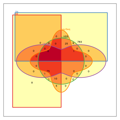 Venn-diagram of the results of all three methods. (FP: are false positives, TN: are true negatives.)
References
- Tian2010
- Linsen2009
- Ozsolak2009
- Meyer2010
- Robinson2010
- Robinson2008
- Anders2010
- Hardcastle2010